Lab 7: Kalman Filter

Drag and Mass Estimations

We can start with approximating the open-loop robot system as first-order using Newton’s second law

$$ F = ma = m\ddot{x} $$

then adding the linear drag force (d) and motor input (u),

$$ F = -d\dot{x} + u $$

the dynamics of the system can be described in terms of second derivative of position

$$ \ddot{x} = -\frac{d}{m} \dot{x} + \frac{u}{m} $$

Then, we can represent the system in state space notation with the state vector

The corresponding dynamics in the state space form

For this system, the drag and mass can be estimated as the1 following lumped parameters covered in lecture

$$ d = \frac{u_{ss}}{\dot{x}_{ss}} $$

$$ m = \frac{-d \cdot t_{0.9}}{\ln(1 - 0.9)} $$

I drove the car at the wall with a PWM value of 120 (in the range of values used for Lab 5) to collect data needed to estimate the above variables. Below are the graphs showing the ToF data and corresponding velocity for the drive at the wall. The velocity was calculated by taking the difference in ToF values over the difference in time for each new ToF data. Data was piped into a CSV for later use via a notification handler with the same structure as used in Lab 5.

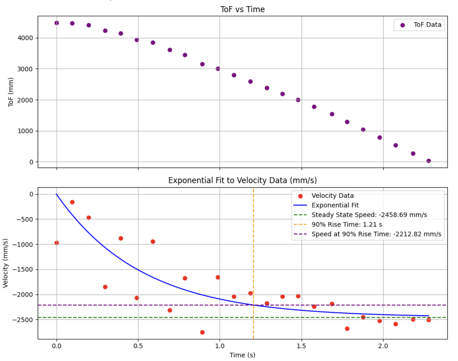
From the steady-state velocity (2.459 m/s), 90% rise time (1.21 s) and speed at 90% rise time (2.213 m/s) printed in the upper right of the graph, as well as setting U to 1 N (unit step) we can now calculate m and d:

$$ d = \frac{1\ \mathrm{N}}{2.459\ \mathrm{m/s}} \approx 0.407\ \mathrm{kg/s} $$

$$ m = \frac{0.407\ \mathrm{kg/s} \cdot 2.213\ \mathrm{m/s}}{\ln(1 - 0.9)} \approx .391\ \mathrm{kg} $$

Finally, we can define our state space matrices in terms of known quantities:

Since we are only directly measuring ToF data X, the state space which will give us that output are the following C and D matrices:

Kalman Python Simulation

Initialize Python KF

For the initial python simulation, the sampling time used for the Kalman filter was 95 ms, the same as my ToF rate. When I confirmed that the simulation was working, I then sped it up to the rate that my PID code loop runs on my arduino (20 ms). U_ss was calculated via u/step_size, where u = 120 and step size = 255. I estimated my ToF variance (dx = 30mm) by taking the average variance in data when statically measuring distance from the wall.

The below code was used to discretize my A and B matrices and define my C and state vector

n = 2  # dimension of the state space
dt = 0.095  # seconds between new readings (set to .02 for high speed)
uss = -0.47 # step input force
dx = 0.03 # ToF variance

Ad = np.eye(n) + dt * A
Bd = dt * B

# Define constants
C = np.array([[1, 0]])
x = np.array([[tof[0]], [0]])  # Initial state using first TOF

Next, I specified my initial process noise and sensor noise covariance matrices via the following equations from lecture.

sig1 = sqrt(100/dt) 
sig2 = sig1
sig3 = sqrt(100/dx)

Sigma_u = np.array([[sig1**2, 0], [0, sig2**2]]) # process noise
Sigma_z = np.array([[sig3**2]]) # measurment noise 

The following code from lecture was used for my Kalman filter

def kalman(mu, sigma, u, y, update = True):
    mu_p = Ad.dot(mu) + Bd.dot(u)
    sigma_p = Ad.dot(sigma.dot(Ad.transpose())) + Sigma_u

    if not update:
        return mu_p, sigma_p

    sigma_m = C.dot(sigma_p.dot(C.transpose())) + Sigma_z
    kkf_gain = sigma_p.dot(C.transpose().dot(np.linalg.inv(sigma_m)))

    y_m = y - C.dot(mu_p)
    mu = mu_p + kkf_gain.dot(y_m)
    sigma = (np.eye(2) - kkf_gain.dot(C)).dot(sigma_p)

    return mu, sigma

Testing KF Simulation (ToF Speed)

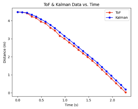
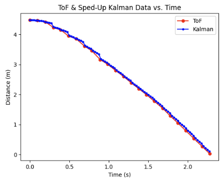
I started with testing the simulation using the variables calculated in the initialization KF section. You can see that the Kalman fit is pretty good– it tracks the ToF well but isn’t so close that it completely disregards the position and velocity from the kalman state dynamics when a new ToF comes in.

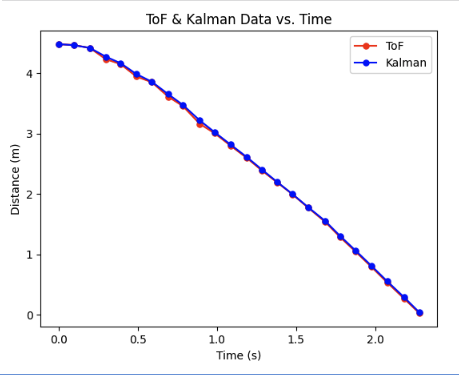
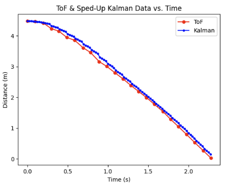
Just for a test, I tried to have my Kalman filter follow my ToF more closely. I achieved this by increasing the $\sigma_1$ and $\sigma_2$ terms which effectively put more trust in the ToF data values. Here is the result of doubling $\sigma_1$ and $\sigma_2$ terms. You can see how closely the Kalman filter tracks the ToF data.

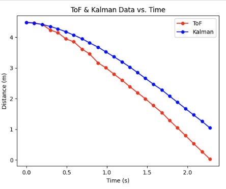
For a final simulation test I wanted to check the other extreme: what happens if I effectively only trust the model? I did this by increasing $\sigma_3$ by an order of 1,000,000 times larger than $\sigma_1$ and $\sigma_2$. You can see in the below graph that the Kalman filter is effectively only using the state space dynamics to predict the next distance value rather than ever meshing with the ToF data.

Testing KF Simulation (PID Speed)

I sped up my dt term to the PID loop speed of 20 ms to simulate how it will run at the faster PID loop speed when integrated onto the robot.

Again, I felt as though my my Kalman values were tracking too close to my ToF, thus I increased $\sigma_3$ to 170 (3x the original value) and left $\sigma_1$ and $\sigma_2$ constant

Onboard Robot Kalman Integration

Initialize Arduino KF

After confirming that the simulation worked as expected, I integrated the code onto my car. The general workflow is as follows:

The below code runs in the main loop without any delays. The pid_start flag is sent over a bluetooth command along with the PID gains. runPIDLin() is responsible for running the Kalman filter and passing the outputs into the PID logic function. After the data arrays are filled they are sent to the computer over artemis by the sendPIDData() function.

if (pid_start) {
  if (counter_lin < lenarr) {
    runPIDLin();
    counter_lin = counter_lin + 1;
  } else {
    sendPIDData();
    Serial.println("data sent");
    stop();
    pid_start = 0;
  }
}

Below is the runPIDLin() function. We can break down each function called

• collectTOF() collects the next ToF value and is responsible for setting the update variable to true dependings on if the ToF value is new or not. The ToF value (new or old) is added to the global TOF1 array.
• kalman() is responsible for running the Kalman filter. Note that the runPIDLin() functions runs as fast as possible thus the kalman filter is especially useful in predicting a distance measurment when new ToF values are not ready. I found that I had to scale my input speed value by 1000 for a better kalman response with from the state space dynamics (this is discussed again at the end).
• pid_speed_ToF() feeds the distance value from the kalman filter into the PID loop which ultimately sends a speed to the motors. Note that the pid_speed_ToF function is effectively the same as from Lab 5.

void runPIDLin() {

  times[counter_lin] = millis();

  // Make sure we have a first ToF value
  while (!kalmanReady) {
    Serial.print("waiting for ToF");
    if (distanceSensor1.checkForDataReady()) {
      kalmanReady = 1;
      collectTOF();
      mu = { TOF1[0], 0 };
      return;
    }
    delay(10);
  }

  collectTOF();

  // If there is new ToF data
  if (update) {
    KalmanResult result = kalman(mu, sigma, Matrix<1, 1>{(pid_speed[counter_lin-1] / 255.0)*1000}, Matrix<1, 1>{TOF1[counter_lin]});
    mu = result.mu;
    sigma = result.sigma;
    pid_speed[counter_lin] = pid_speed_ToF(Kp, Ki, Kd, mu(0, 0), target_tof);
    kf[counter_lin] = mu(0, 0);
    update = 0;
  }

  // If no new ToF data
  else {
    /// Same as above except pass in false for fifth kalman() parameter to flip update to false
    ...
  }
  // Update Data arrays to send over bluetooth
  ...
}

Here is the kalman() function. Note that the inverse and transpose functions had to be swapped out for Arduino alternatives

struct KalmanResult {
  Matrix<2, 1> mu;
  Matrix<2, 2> sigma;
};

KalmanResult kalman(Matrix<2, 1> mu_in, Matrix<2, 2> sigma_in, Matrix<1, 1> u, Matrix<1, 1> y, bool update = true) {
  Matrix<2, 1> mu_p = Ad * mu_in + Bd * u;
  Matrix<2, 2> sigma_p = Ad * (sigma_in * ~Ad) + Sigma_u; // ~ used for trasnspose

  if (!update) {
    return { mu_p, sigma_p };
  }

  Matrix<1, 1> sigma_m = C * sigma_p * ~C + Sigma_z;
  Matrix<1, 1> sigma_m_inv = { 1 / sigma_m(0) }; // scalar inverse used
  Matrix<2, 1> kkf_gain = sigma_p * ~C * sigma_m_inv;

  float y_m = y(0, 0) - (C * mu_p)(0, 0);
  Matrix<2, 1> mu = mu_p + kkf_gain * y_m;
  Matrix<2, 2> sigma = (I - kkf_gain * C) * sigma_p;

  return { mu, sigma };
}

Test Arduino

There was extensive debugging required to implement the Kalman filter onto the robot. I will be showing three test cases in this section to summarize all of the robot integration work and results.

1. I started by testing the Kalman filter state dynamics similar to how the kalman dynamics model was tested in the python simulation. I did this by effectively putting zero trust in my ToF data relative to my dynamics model by making $\sigma_3$ an order of 1,000,000 times larger than $\sigma_1$ and $\sigma_2$. This yielded the following graph which proves that the Kalman filter is standalone and independent– it properly follows the system dynamics derived at the beginning of the lab when not fusing the Kalman predicted values with ToF.

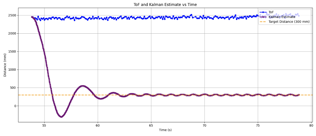
2. I implemented proportional control and ran the robot at a wall with the target of stopping 300 mm (~1ft) away. With only proportional control, I was unable to avoid hitting the wall unless the robot went extremely slow. Here is a trial where the robot does hit the wall but is able to bounce off and still meet the 1 ft target. Note that the speed is constant (horizontal) during some of the run due to the speed floor that is implemented. You can also see the speed ceiling in the PD control at the beginning.

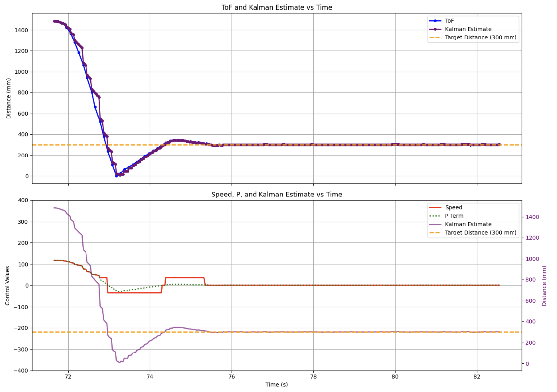
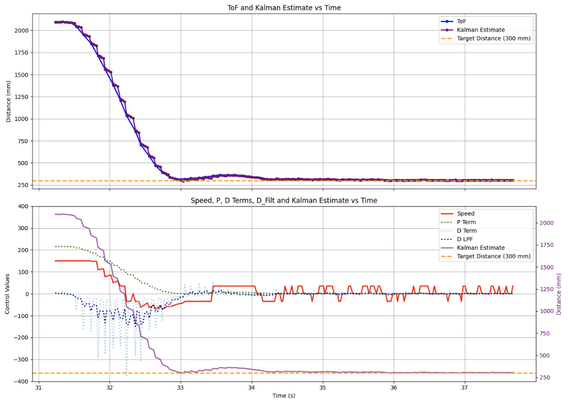
3. The PD Control worked really well. Relative to the proportional control above, you can see that the rise time does slightly increase as the derivative term is helping to slow the car down earlier, but it allows for effectively zero overshoot. If I continued to increase the proportional and derivative gains, I might have been able to achieve a similarly quick rise time with the derivative term still reducing overshoot. The robot stopped right about 1 ft away from the wall with little steady state error; as in previous labs, an integral term did not seem to be needed. You can see the implementation of a low pass filter to reduce derivative kick and overall noise spikes. From the graph you can see that the Kalman filter follows the ToF data fairly well and, as proved above, is able to make its own predicitions using the state dynamcis which is especially useful when new ToF data isn’t ready.

Variable Discussion

Quick recap of variables used to tune and their impacts:

• m and d: Although these parameters were derived from experimentally determined variables at the start, they can still be fine-tuned. A higher value of m corresponds to a car with greater inertia; it accelerates less in response to a control input. The d term mainly influences the max speed of the car (calculated by the Kalman filter) and how rapidly the speed decreases once the control input is removed.
• u: The control input, unlike the m and d terms, come directly from the PID controller and in theory probably should not be changed in order to tune the kalman filter. However, I found that scaling/ampliyfing it (as mentioned earlier in the lab) was a quick and effective workaround to better match the filter’s expected behavior.
• $\boldsymbol{\sigma}$: As previously mentioned in the lab, $\sigma_1$ and $\sigma_2$ represent the “trust” in the ToF data realitve to the model. For example, large $\sigma_1$ and $\sigma_2$ correspond to low confidence in the model’s predictions and make the filter rely more heavily on sensor measurments. $\sigma_3$ is effectively the same but for the model. Large $\sigma_3$ values represent more trust in the model than in the ToF measurments.

Collaboration

I collaborated extensively on this project with Jack Long and Trevor Dales. I referenced Stephan Wagner’s site with help in implementing the python kalman simulation! ChatGPT was used to help plot graphs.